I Python, You R, We Julia

When we decided to rename part of the IPython project to Jupyter in 2014, we had many good reasons. Our goal was to make (Data)Science and Education better, by providing Free and Open-Source tools that can be used by everyone. The name “Jupyter” is a strong reference to Galileo, who detailed his discovery of the Moons of Jupiter in his astronomical notebooks. The name is also a play on the languages Julia, Python, and R, which are pillars of the modern scientific world. While we ❤️🐍(Love Python), and use it for much of the architecture in Jupyter, we believe that all open-source languages have an important role in scientific and data analysis workflows. We have strived to make Jupyter a platform that treats all open-source languages as first-class citizens.

You may know that Jupyter has several dozen kernels in as many languages, and that you can choose any of them to power the code execution in a single notebook. However, the possibilities for cross-language integration go way beyond this, which I’ll attempt to demonstrate here.

What I’ll describe below has been possible for now several years – from even before the name Jupyter was first mentioned. It relies on the work of many Open Source libraries, too many to cite all the authors. It is not the only solution — neither the first, not the last. RStudio recently blogged about reticulate, which allows you to intertwine Python and R code. BeakerX is also another solution that appears to to support many languages.

We hope that showing how multiple languages can be use together will help make you more efficient in your work, and that it promotes cooperation across our communities to use the strengths of each language. This article only scratches the surface, you can read more in depth what you can do and how this works in a notebook I wrote some time ago.

Follow along on Binder

We created Jupyter and Binder to make science more trustworthy and allow results to be replicate. If you doubt what I have written below, or just want to follow along feel free to try on your own using Binder — the docker image is quite big so can take a while to launch. In the linked notebook we show a couple of extra languages.

The Tail of Fibonacci

A famous example of recursion in Computer Science is the Fibonacci series, its ubiquity allows the reader not to focus on the sequence itself but on the environment around it. As a reminder, the Fib sequence is defined with its first two terms being one, then each subsequent term as the sum of the two preceding terms; i.e F(1)= 1, F(2)=1, F(n) = F(n-1)+F(n-2)

We can calculate the first few terms: 1, 1, 2, 3, 5, 8 … note that F(5) is a fixed point F(5) = 5, and trust that asymptotically the sequence behaves like exp(n).

Let’s see how one can use many languages to play with fibonacci.

I, Python

For this exploration we’ll start with Python. It is my language of choice, the one I’m the most familiar with:

def fib(n):
    """
    A simple definition of fibonacci manually unrolled
    """
    if n<2:
        return 1
    x,y = 1,1
    for i in range(n-2):
        x,y = y,x+y
    return y

We can check that the fib function works correctly.

>>> [fib(i) for i in range(1,10)]
[1, 1, 2, 3, 5, 8, 13, 21, 34]

And plot it:

%matplotlib inline
import numpy as np
X = np.arange(1,30)
Y = np.array([fib(x) for x in X])
import matplotlib.pyplot as plt
fig, ax = plt.subplots()
ax.scatter(X, Y)
ax.set(xlabel='n', ylabel='fib(n)',
       title='The Fibonacci sequence grows fast !')

As you can see it grows quite quickly, actually it’s exponential. Now let’s see how we can check this exponential behavior using multi-language integration.

You R

With the fantastic RPy2 package, we can integrate code seamlessly between Python and R, allowing you to send data back and forth between the two languages. RPy2 will translate R data structures to Python and NumPy, and vice versa.

In addition, RPy2 has extra integration with IPython and provides “Magics” to write inline or multiline R code. Loading the RPy2 extension exposes the %R , %%R, %Rpush and %%Rpull commands for writing R.

%load_ext rpy2.ipython

We can use %RPush to send data to a stateful R process.

%Rpush Y X

and use %%R in order to instruct the R process to run an R cell.

%%R
my_summary = summary(lm(log(Y)~X))
val <- my_summary$coefficients

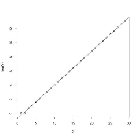
plot(X, log(Y))
abline(my_summary)

Here we make a linear regression model on log(Y) vs X. As Y is (hopefully) exponential, we should get a nice line. RPy2 provides rich display integration which will nicely display outputs and plots inline in a notebook:

We can of course ask for the linear regression summary:

%%R
my_summary

Which outputs:

Call:
lm(formula = log(Y) ~ X)

Residuals:
      Min        1Q    Median        3Q       Max 
-0.183663 -0.013497 -0.004137  0.006046  0.296094 

Coefficients:
             Estimate Std. Error t value Pr(>|t|)    
(Intercept) -0.775851   0.026173  -29.64   <2e-16 ***
X            0.479757   0.001524  314.84   <2e-16 ***
---
Signif. codes:  0 ‘***’ 0.001 ‘**’ 0.01 ‘*’ 0.05 ‘.’ 0.1 ‘ ’ 1

Residual standard error: 0.06866 on 27 degrees of freedom
Multiple R-squared:  0.9997,	Adjusted R-squared:  0.9997 
F-statistic: 9.912e+04 on 1 and 27 DF,  p-value: < 2.2e-16

We can also lift the results from R to Python using %Rget:

coefs = %Rget val
y0,k = coefs.T[0:2]
y0,k

Which yields

(-0.77585097534858738, 0.4797570904348315)

Here we saw that RPy2 allows us to pass data back and forth between Python and R; This is incredibly useful to leverage the strengths of each language. This is a toy example, but you could imagine using various python libraries to get data from servers, and move to R for the statistical analysis.

However, sometime moving data between languages may be too limiting. Let’s see how we can leverage the same mechanism to gain some performance, by integrating with a lower level language.

Let’s C

Python and R are not the most performant languages for pure numerical speed. When performance improvement is necessary, developers tend to utilize compiled language like C/C++/Fortran.

Unfortunately, compiled languages generally have a poor interactive experience, and where CPU cycles are gained, human developer time may be lost.

Using magics, we can, as we did for R, include snippets of C, Cython, Fortran, Rust … and many other languages.

import cffi_magic
%%cffi int cfib(int);

int cfib(int n)
{
    int res=0;
    if (n <= 2){  
        res = 1;
    } else {
        res = cfib(n-1)+cfib(n-2);
    }
    return res;
}

We can interactively redefine this function, and it will magically appear on the Python namespace. It works identically to the fib we defined earlier, but is much faster. Note that the Python Fib, and C fib time here are difficult to compare as the C one is recursive (behave in O(exp(n)))and the Python one is hand unrolled, so behave in O(n) .

More technical details can be found in a notebook I wrote earlier, but the same can be done with other languages that call one another, and lines like the following work perfectly:

assert py_fib(cython_fib(c_fib(fortran_fib(rust_fib(5)))) == 5

Julia to bind them all

The last example is a technical marvel that was first developed by Steven Johnson and Fernando Pérez, it relies on starting a Julia and Python interpreter together, allowing them to share memory. This allow both languages not only to exchange data and functions, but to manipulate live object references from the other interpreter. Extra integration with IPython via magics allows us to run inline Julia in Python (%julia, %%julia), while Julia Macros (@pyimport) allows python code to be run from within Julia.

Below we’ll show integration with Graphing libraries (matplotlib), so let’s set up our environment.

%matplotlib inline
%load_ext julia.magic

We’ll start from within Julia, and import a few python packages:

%julia @pyimport matplotlib.pyplot as plt
%julia @pyimport numpy as np

We now have access – from within Julia – to matplotlib and numpy. We can now seamlessly integrate Julia native numerical capabilities and functions with our Python kernel.

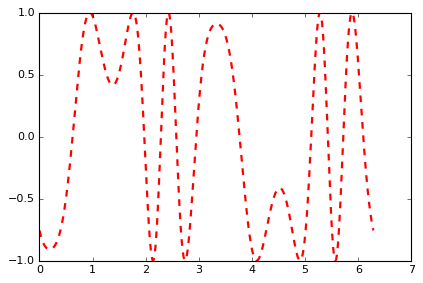
%%julia                                        
t = linspace(0, 2*pi,1000);             
s = sin(3*t + 4*np.cos(2*t));           
fig = plt.gcf()                         
plt.plot(t, s, color="red", linewidth=2.0, linestyle="--", label="sin(3t+4.cos(2t))")

Note that in above block, t, pi are native julia; s is computed via sin (julia), t (julia), cos (numpy); fig is a Python object. As the Julia Magic provides IPython display integration, the code above displays this nice graph.

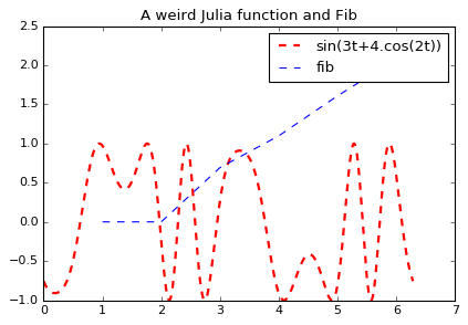
We now want to annotate this graph from Python, as the API is more convenient:

import numpy as np
fig = %julia fig
fig.axes[0].plot(X[:6], np.log(Y[:6]), '--', label='fib')
fig.axes[0].set_title('A weird Julia function and Fib')
fig.axes[0].legend()
fig

After passing a reference to fig from Julia to Python, we can annotate it (and plot one of the fib functions we defined earlier in C, Fortran, Rust, etc…)

Here we can see that unlike BeakerX, R-Reticular or RPy2, we are actually sharing live objects, and can manipulate them from both languages. But let’s push things a bit further.

The fib function can be defined recursively; let’s have some fun and define a pyfib function in Python that recurses via the a jlfib function in Julia. Meanwhile, the jlfib function in Julia recurses using the python function. We’ll print (J , or (P when switching language:

jlfib = %julia _fib(n, pyfib) = n <= 2 ? 1 : pyfib(n-1, _fib) + pyfib(n-2, _fib)


def pyfib(n, _fib):
    print('(P', end='')
    if n <= 2:
         r = 1
    else:
        print('(J', end='')
        # here we tell julia (_fib) to recurse using Python
        r =  _fib(n-1, pyfib) + _fib(n-2, pyfib)
        print(')',end='')
    print(')',end='')
    return r
fibonacci = lambda x: pyfib(x, jlfib)
fibonacci(10)

We can now transparently call the function :

(P(J(P(J(P(J(P(J(P)(P)))(P(J))(P(J))(P)))(P(J(P(J))(P)(P)(P)))(P(J(P(J))(P)(P)(P)))(P(J(P)(P)))))(P(J(P(J(P(J))(P)(P)(P)))(P(J(P)(P)))(P(J(P)(P)))(P(J))))(P(J(P(J(P(J))(P)(P)(P)))(P(J(P)(P)))(P(J(P)(P)))(P(J))))(P(J(P(J(P)(P)))(P(J))(P(J))(P)))))
55

If you are interested in diving more into details see this post from a couple of years ago with all the actual code.

I hope that this post has convinced you that Jupyter – via the IPython kernel – has deep cross-language integration (and has had this for many years). I also hope it lifted the misconception in that in Jupyter “1 kernel == 1 language” or even that “1 notebook == 1 language”. Each of the approaches shown here (as well as Reticulate, BeakerX, etc) have their pros and cons. Use the approach that fits your needs and makes your workflow efficient, regardless of the tool, language, or libraries you use.